In this tutorial we will learn the following features:
Design a training scheme composed of two cascaded networks.
Visualize the training with tensorboard.
Generate a GIF to visualize the learning of the model.
Find the optimal threshold to binarize images based on the validation sub-dataset.
In our example, the model will first locate the spinal cord (step 1). This localisation will then be used to crop the images around this region of interest, before segmenting the cerebrospinal fluid (CSF, step 2).
A dataset example is available for this tutorial. If not already done, download the dataset with the following line.
For more details on this dataset see One-class segmentation with 2D U-Net.
# Download data
ivadomed_download_data-ddata_example_spinegeneric
In ivadomed, training is orchestrated by a configuration file. Examples of configuration files are available in
the ivadomed/config/ and the documentation is available in Configuration File.
In this tutorial we will use the configuration file: ivadomed/config/config.json.
First off, copy this configuration file in your local directory to avoid modifying the source file:
cp<PATH_TO_IVADOMED>/ivadomed/config/config.json.
Then, open it with a text editor. Which you can view directly here: or you can see it in the collapsed JSON code block below.
From this point onward, we will discuss some of the key parameters to use cascaded models. Most parameters are configurable only via modification of the configuration JSONfile.
For those that supports commandline run time configuration, we included the respective command versions under the CommandLineInterface tab
At this line in the config.json is where you can update the debugging.
debugging: Boolean, create extended verbosity and intermediate outputs. Here we will look at the intermediate predictions
with tensorboard, we therefore need to activate those intermediate outputs.
"debugging":true
At this line in the config.json is where you can update the object_detection_path within the object_detection_params sub-dictionary.
object_detection_params:object_detection_path: Location of the object detection model. This parameter corresponds
to the path of the first model from the cascaded architecture that segments the spinal cord. The packaged model in the
downloaded dataset located in the folder trained_model/seg_sc_t1-t2-t2s-mt will be used to detect the spinal cord.
This spinal cord segmentation model will be applied to the images and a bounding box will be created around this mask
to crop the image.
At this line in the config.json is where you can update the safety_factor within the object_detection_params sub-dictionary.
object_detection_params:safety_factor: Multiplicative factor to apply to each dimension of the bounding box. To
ensure all the CSF is included, a safety factor should be applied to the bounding box generated from the spinal cord.
A safety factor of 200% on each dimension is applied on the height and width of the image. The original depth of the
bounding box is kept since the CSF should not be present past this border.
"safety_factor":[2,2,1]
At this line in the config.json is where you can update the target_suffix within the loader_parameters sub-dictionary.
loader_parameters:target_suffix: Suffix of the ground truth segmentation. The ground truth are located under the
DATASET/derivatives/labels folder. The suffix for CSF labels in this dataset is _csfseg-manual:
"target_suffix":["_csfseg-manual"]
At this line in the config.json is where you can update the contrast_params within the loader_parameters sub-dictionary.
loader_parameters:contrast_params: Contrast(s) of interest. The CSF labels are only available in T2w contrast in
the example dataset.
At this line in the config.json is where you can update the size within the transformation:CenterCrop sub-dictionary.
transformation:CenterCrop:size: Crop size in voxel. Images will be cropped or padded to fit these dimensions. This
allows all the images to have the same size during training. Since the images will be cropped around the spinal cord,
the image size can be reduced to avoid large zero padding.
Once the configuration file is ready, run the training. ivadomed has an option to find a threshold value which optimized the dice score on the validation dataset. This threshold will be further used to binarize the predictions on testing data. Add the flag -t with an increment
between 0 and 1 to perform this threshold optimization (i.e. -t0.1 will return the best threshold between 0.1,
0.2, …, 0.9)
To help visualize the training, the flag --gif or -g can be used. The flag should be followed by the number of
slices by epoch to visualize. For example, -g2 will generate 2 GIFs of 2 randomly selected slices from the
validation set.
Make sure to run the CLI command with the --train flag, and to point to the location of the dataset via the flag --path-datapath/to/bids/data.
If the flag --gif or -g was used, the training can be visualized through gifs located in the folder specified by the --path-output flag
<PATH_TO_OUT_DIR>/gifs.
Another way to visualize the training is to use Tensorboard. Tensorboard helps to visualize the augmented input images,
the model’s prediction, the ground truth, the learning curves, and more. To access this data during or after training,
use the following command-line:
tensorboard--logdir<PATH_TO_OUT_DIR>
The following should be displayed in the terminal:
Serving TensorBoard on localhost; to expose to the network, use a proxy or pass --bind_allTensorBoard 2.2.1 at http://localhost:6006/ (Press CTRL+C to quit)
Open your browser and type the URL provided, in this case http://localhost:6006/.
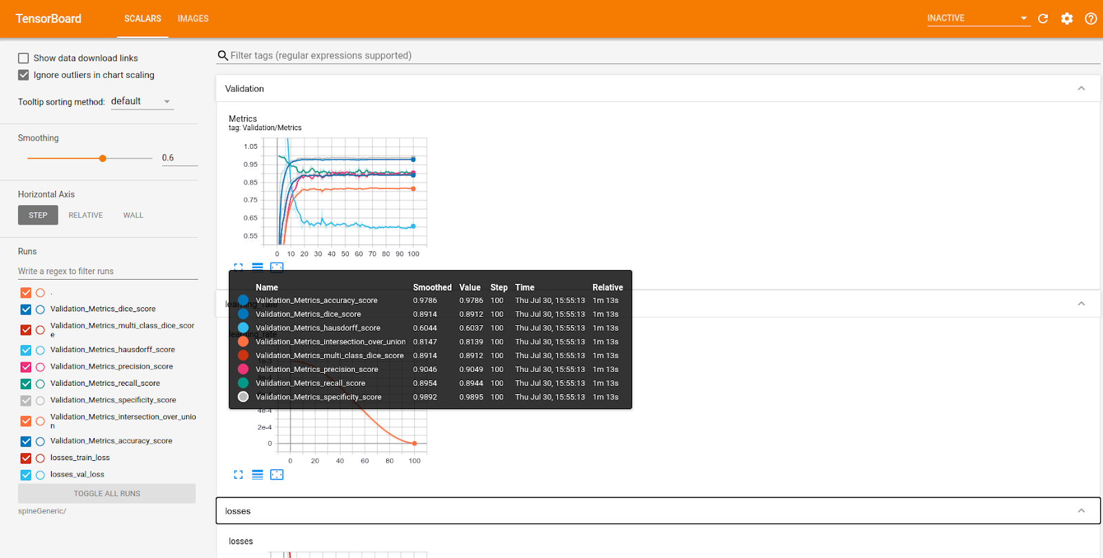
In the scalars folder, the evolution of metrics, learning rate and loss through the epochs can be visualized.
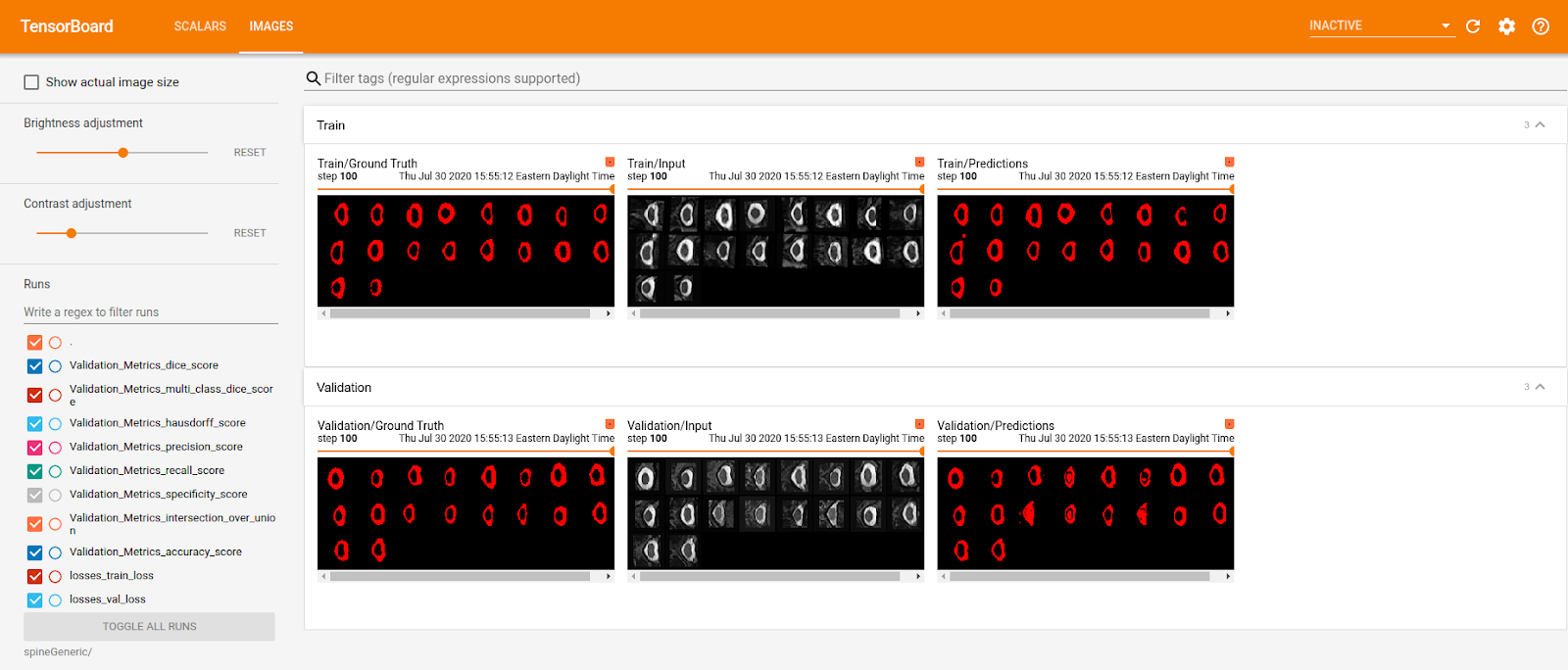
In the image folder, the training and validation ground truth, input images and predictions are displayed. With this
feature, it is possible to visualize the cropping from the first model and confirm that the spinal cord
was correctly located.
postprocessing:binarize_prediction: Threshold at which predictions are binarized. Before testing the model,
modify the binarization threshold to have a threshold adapted to the data: