One-class segmentation with 2D U-Net
In this tutorial we will learn the following features:
Training of a segmentation model (U-Net 2D) with a single label on multiple contrasts,
Testing of a trained model and computation of 3D evaluation metrics.
Visualization of the outputs of a trained model.
An interactive Colab version of this tutorial is directly accessible here:
Download dataset
We will use a publicly-available dataset consisting of MRI data of the spinal cord. This dataset is a subset of the spine-generic multi-center dataset and has been pre-processed to facilitate training/testing of a new model. Namely, for each subject, all six contrasts were co-registered together. Semi-manual cord segmentation for all modalities and manual cerebrospinal fluid labels for T2w modality were created. More details here.
In addition to the MRI data, this sample dataset also includes a trained model for spinal cord segmentation.
To download the dataset (~490MB), run the following commands in your terminal:
# Download data
ivadomed_download_data -d data_example_spinegeneric
Configuration file
In
ivadomed, training is orchestrated by a configuration file. Examples of configuration files are available in theivadomed/config/folder and the documentation is available in Configuration File.In this tutorial we will use the configuration file:
ivadomed/config/config.json. First off, copy this configuration file in your local directory (to avoid modifying the source file):cp <PATH_TO_IVADOMED>/ivadomed/config/config.json .Then, open it with a text editor. Which you can view directly here: or you can see it in the collapsed JSON code block below.
From this point onward, we will discuss some of the key parameters to perform a one-class 2D segmentation training. Most parameters are configurable only via modification of the configuration
JSON file. For those that supports command line run time configuration, we included the respective command versions under theCommand Line Interfacetab
command: Action to perform. Here, we want to train a model:
path_output: Folder name that will contain the output files (e.g., trained model, predictions, results).
loader_parameters:path_data: Location of the dataset. As discussed in Data, the dataset should conform to the BIDS standard. Modify the path so it points to the location of the downloaded dataset.
loader_parameters:target_suffix: Suffix of the ground truth segmentation. The ground truth is located under theDATASET/derivatives/labelsfolder. In our case, the suffix is_seg-manual:At this line in the
config.jsonis where you can update thetarget_suffixwithin theloader_parameterssub-dictionary."target_suffix": ["_seg-manual"]
loader_parameters:contrast_params: Contrast(s) of interestAt this line in the
config.jsonis where you can update thecontrast_paramssub-dictionary within theloader_parameterssub-dictionary."contrast_params": { "training_validation": ["T1w", "T2w", "T2star"], "testing": ["T1w", "T2w", "T2star"], "balance": {} }
loader_parameters:slice_axis: Orientation of the 2D slice to use with the model.At this line in the
config.jsonis where you can update theslice_axissubkey within theloader_parameterssub-dictionary."slice_axis": "axial"
loader_parameters:multichannel: Turn on/off multi-channel training. Iftrue, each sample has several channels, where each channel is an image contrast. Iffalse, only one image contrast is used per sample.At this line in the
config.jsonis where you can update themultichannelsubkey within theloader_parameterssub-dictionary."multichannel": falseNote
The multichannel approach requires that for each subject, the image contrasts are co-registered. This implies that a ground truth segmentation is aligned with all contrasts, for a given subject. In this tutorial, only one channel will be used.
training_parameters:training_time:num_epochs: the maximum number of epochs that will be run during training. Each epoch is composed of a training part and an evaluation part. It should be a strictly positive integer.At this line in the
config.jsonis where you can update thenum_epochssubkey within thetraining_parameters:training_timesub-dictionary."num_epochs": 100
Train model
Once the configuration file is ready, run the training:
ivadomed --train -c config.json --path-data path/to/bids/data --path-output path/to/output/directory
In the above command, we execute the
--traincommand and manually specified--path-dataand--path-outputand overwrote/replace the specification inconfig.json
--train: We can pass other flags to execute different commands (training, testing, segmentation), see Usage.
--path-output: Folder name that will contain the output files (e.g., trained model, predictions, results).
--path-data: Location of the dataset. As discussed in Data, the dataset should conform to the BIDS standard. Modify the path so it points to the location of the downloaded dataset.If you set the
command,path_output, andpath_dataarguments in your config file, you do not need to pass the above the specific CLI flags.Instead, make the following changes to the JSON file at the specific lines:
Command parameter located here
"command": "train"Path output parameter located here
"path_output": "spineGeneric"
path-output: Folder name that will contain the output files (e.g., trained model, predictions, results).Path Data located here
"path_data": "data_example_spinegeneric"
path-data: Location of the dataset. As discussed in Data, the dataset should conform to the BIDS standard. Modify the path so it points to the location of the downloaded dataset.Then execute the following simplified command:
ivadomed -c config.jsonNote
If a compatible GPU is available, it will be used by default. Otherwise, training will use the CPU, which will take a prohibitively long computational time (several hours).
The main parameters of the training scheme and model will be displayed on the terminal, followed by the loss value on training and validation sets at every epoch. To know more about the meaning of each parameter, go to Configuration File. The value of the loss should decrease during the training.
Creating output path: spineGeneric
Cuda is not available.
Working on cpu.

Selected architecture: Unet, with the following parameters:
dropout_rate: 0.3
bn_momentum: 0.1
depth: 3
is_2d: True
final_activation: sigmoid
folder_name: my_model
in_channel: 1
out_channel: 1
Dataframe has been saved in spineGeneric\bids_dataframe.csv.
After splitting: train, validation and test fractions are respectively 0.6, 0.2 and 0.2 of participant_id.

Selected transformations for the ['training'] dataset:
Resample: {'hspace': 0.75, 'wspace': 0.75, 'dspace': 1}
CenterCrop: {'size': [128, 128]}
RandomAffine: {'degrees': 5, 'scale': [0.1, 0.1], 'translate': [0.03, 0.03], 'applied_to': ['im', 'gt']}
ElasticTransform: {'alpha_range': [28.0, 30.0], 'sigma_range': [3.5, 4.5], 'p': 0.1, 'applied_to': ['im', 'gt']}
NumpyToTensor: {}
NormalizeInstance: {'applied_to': ['im']}

Selected transformations for the ['validation'] dataset:
Resample: {'hspace': 0.75, 'wspace': 0.75, 'dspace': 1}
CenterCrop: {'size': [128, 128]}
NumpyToTensor: {}
NormalizeInstance: {'applied_to': ['im']}
Loading dataset: 100%|██████████████████████████████████████████████████████████████████████████████████████████████████████████████████████████████████████████████████████████████████████████████████████████████████| 6/6 [00:00<00:00, 383.65it/s]
Loaded 92 axial slices for the validation set.
Loading dataset: 100%|████████████████████████████████████████████████████████████████████████████████████████████████████████████████████████████████████████████████████████████████████████████████████████████████| 17/17 [00:00<00:00, 282.10it/s]
Loaded 276 axial slices for the training set.
Creating model directory: spineGeneric\my_model

Initialising model's weights from scratch.

Scheduler parameters: {'name': 'CosineAnnealingLR', 'base_lr': 1e-05, 'max_lr': 0.01}

Selected Loss: DiceLoss
with the parameters: []
Epoch 1 training loss: -0.0336.
Epoch 1 validation loss: -0.0382.
After 100 epochs (see
num_epochsin the configuration file), the Dice score on the validation set should be ~90%.
Evaluate model
To test the trained model on the testing sub-dataset and compute evaluation metrics, run:
ivadomed --test -c config.json --path-data path/to/bids/data --path-output path/to/output/directoryIf you prefer to use config files over CLI flags, set
commandtotestin the following line in you config file:"command": "test"You can also set
path_output, andpath_dataarguments in theconfig.jsonrespectively.Then run:
ivadomed -c config.jsonThe model’s parameters will be displayed in the terminal, followed by a preview of the results for each image. The resulting segmentation is saved for each image in the
<PATH_TO_OUT_DIR>/pred_maskswhile a csv file, saved in<PATH_TO_OUT_DIR>/results_eval/evaluation_3Dmetrics.csv, contains all the evaluation metrics. For more details on the evaluation metrics, seeivadomed.metrics.Output path already exists: spineGeneric Cuda is not available. Working on cpu. Selected architecture: Unet, with the following parameters: dropout_rate: 0.3 bn_momentum: 0.1 depth: 3 is_2d: True final_activation: sigmoid folder_name: my_model in_channel: 1 out_channel: 1 Dataframe has been saved in spineGeneric\bids_dataframe.csv. After splitting: train, validation and test fractions are respectively 0.6, 0.2 and 0.2 of participant_id. Selected transformations for the ['testing'] dataset: Resample: {'hspace': 0.75, 'wspace': 0.75, 'dspace': 1} CenterCrop: {'size': [128, 128]} NumpyToTensor: {} NormalizeInstance: {'applied_to': ['im']} Loading dataset: 100%|██████████████████████████████████████████████████████████████████████████████████████████████████████████████████████████████████████████████████████████████████████████████████████████████████| 6/6 [00:00<00:00, 373.59it/s] Loaded 94 axial slices for the testing set. Loading model: spineGeneric\best_model.pt Inference - Iteration 0: 100%|███████████████████████████████████████████████████████████████████████████████████████████████████████████████████████████████████████████████████████████████████████████████████████████| 6/6 [00:29<00:00, 4.86s/it] {'dice_score': 0.9334570551249012, 'multi_class_dice_score': 0.9334570551249012, 'precision_score': 0.925126264682505, 'recall_score': 0.9428409070673442, 'specificity_score': 0.9999025807354961, 'intersection_over_union': 0.8756498644456311, 'accu racy_score': 0.9998261755671077, 'hausdorff_score': 0.05965616760384793} Run Evaluation on spineGeneric\pred_masks Evaluation: 100%|████████████████████████████████████████████████████████████████████████████████████████████████████████████████████████████████████████████████████████████████████████████████████████████████████████| 6/6 [00:05<00:00, 1.04it/s] avd_class0 dice_class0 lfdr_101-INFvox_class0 lfdr_class0 ltpr_101-INFvox_class0 ltpr_class0 mse_class0 ... n_pred_class0 precision_class0 recall_class0 rvd_class0 specificity_class0 vol_gt_class0 vol_pred_class0 image_id ... sub-mpicbs06_T1w 0.086296 0.940116 0.0 0.0 1.0 1.0 0.002292 ... 1.0 0.902774 0.980680 -0.086296 0.999879 4852.499537 5271.249497 sub-mpicbs06_T2star 0.038346 0.909164 0.0 0.0 1.0 1.0 0.003195 ... 1.0 0.892377 0.926595 -0.038346 0.999871 4563.749565 4738.749548 sub-mpicbs06_T2w 0.032715 0.947155 0.0 0.0 1.0 1.0 0.001971 ... 1.0 0.932153 0.962648 -0.032715 0.999920 4852.499537 5011.249522 sub-unf01_T1w 0.020288 0.954007 0.0 0.0 1.0 1.0 0.002164 ... 1.0 0.944522 0.963684 -0.020288 0.999917 6161.249412 6286.249400 sub-unf01_T2star 0.001517 0.935124 0.0 0.0 1.0 1.0 0.002831 ... 1.0 0.934416 0.935834 -0.001517 0.999904 5766.249450 5774.999449 [5 rows x 16 columns]The test image segmentations are stored in
<PATH_TO_OUT_DIR>/pred_masks/and have the same name as the input image with the suffix_pred. To visualize the segmentation of a given subject, you can use any NIfTI image viewer. For FSLeyes users, this command will open the input image with the overlaid prediction (segmentation) for one of the test subject:fsleyes <PATH_TO_BIDS_DATA>/sub-mpicbs06/anat/sub-mpicbs06_T2w.nii.gz <PATH_TO_OUT_DIR>/pred_masks/sub-mpicbs06_T2w_pred.nii.gz -cm redAfter the training for 100 epochs, the segmentations should be similar to the one presented in the following image. The output and ground truth segmentations of the spinal cord are presented in red (subject
sub-mpicbs06with contrast T2w):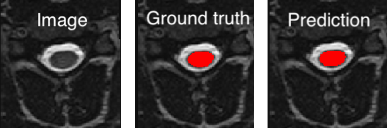
Another set of test image segmentations are also present in <PATH_TO_OUT_DIR>/pred_masks/ with the suffix _pred-TP-FP-FN when the evaluation_parameters:object_detection_metrics is set to true (Default: true). These files include 3 possible values depending if each object detected in the prediction compared to the ground-truth is a True Positive (TP), False Positive (FP) or False Negative (FN). In NIfTI files (.nii.gz), the respective values for TP, FP and FN are 1, 2 and 3.